Quick 2D Prototyping With Gpytoolbox III: Distances to 2D Polylines
Gpytoolbox version 0.1.0 has just been released!! You can install it directly through pip:
pip install gpytoolbox
This is the third in a series of blogposts highlighting features of our newly released library. You can find rest of the blog entries here. Today, we are looking at how to compute distances to 2D polylines.
There are many reasons why you may want to compute the minimum distance from a given point in 2D to a polyline: for example, to guide sampling or as a stopping criterion in iterative algorithms. Gpytoolbox provides a breadth of tools for computing distances to fit different needs.
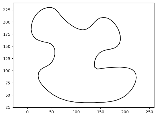
Let’s start by loading a polyline and computing a single point’s distance to it:
# load polyline
from gpytoolbox import png2poly, edge_indices
poly = png2poly("illustrator.png")
vertices = poly[0]
# Downsample the polyline for simplicity
vertices = vertices[::10,:]
edges = edge_indices(vertices.shape[0], closed=True)
import matplotlib.pyplot as plt
_ = plt.plot(vertices[:, 0], vertices[:, 1], '-k')
_ = plt.axis('equal')
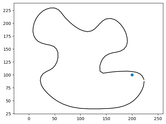
# Consider a poing in space
point = np.array([200,100])
# Visualize it
_ = plt.plot(point[0], point[1], 'o')
_ = plt.plot(vertices[:, 0], vertices[:, 1], '-k')
_ = plt.axis('equal')
# Now, we call the function that computes its squared distance to the polyline
from gpytoolbox import squared_distance
sqrd, ind, t = squared_distance(point, vertices, F=edges)
print("The distance is ", float(np.sqrt(sqrd)))
The distance is 6.1621198369606835
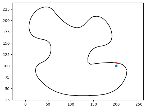
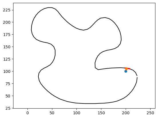
squared_distance not only returns the value of the distance, it also includes very useful information. For example, it tells us the polyline edge that is the closest to our point:
# Plot the polyline and the closest edge
_ = plt.plot(vertices[:, 0], vertices[:, 1], '-k')
# Get the vertices of the closest edge
vertices_of_closest_edge = vertices[edges[ind,:],:].squeeze()
_ = plt.plot(vertices_of_closest_edge[:,0], vertices_of_closest_edge[:,1], '-r', linewidth=3)
_ = plt.plot(point[0], point[1], 'o')
_ = plt.axis('equal')
It also includes a parameter t, that tells us where along that edge the closest polyline point lays. We can use it to calculate said closest point:
# Find the closest point on the polyline
closest_point = vertices[edges[ind,0],:] + (1-t) * (vertices[edges[ind,1],:] - vertices[edges[ind,0],:])
closest_point = closest_point.squeeze()
print("The closest point is ", closest_point)
# Plot the polyline and the closest point
_ = plt.plot(vertices[:, 0], vertices[:, 1], '-k')
_ = plt.plot(point[0], point[1], 'o')
_ = plt.plot(vertices_of_closest_edge[:,0], vertices_of_closest_edge[:,1], '-r', linewidth=3)
_ = plt.plot(closest_point[0], closest_point[1], 'o')
_ = plt.axis('equal')
The closest point is [200.97159662 105.31480424]
Using squared_distance we can find the distance of many points to the polyline at the same time:
# Often, it helps to normalize the polyline
from gpytoolbox import normalize_points
vertices = normalize_points(vertices)
# Generate many random points
points = np.random.rand(1000,2)-0.5
# Compute the squared distance to the polyline
sqrd, ind, t = squared_distance(points, vertices, F=edges)
# Plot the polyline and the points
_ = plt.plot(vertices[:, 0], vertices[:, 1], '-k')
# Plot points with sqrd as color
_ = plt.scatter(points[:,0], points[:,1], c=sqrd)
_ = plt.colorbar()
_ = plt.axis('equal')
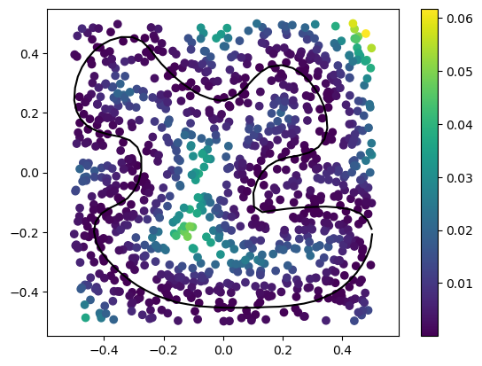
You may have noticed that computation took some time. That’s because, for each point in the set, squared_distance is going through every single edge in the polyline to check if it’s the closest. This performance hit will be significant, especially if the shape is very complex:
# Let's begin by loading the image into a polyline
from gpytoolbox import png2poly, edge_indices
poly = png2poly("switzerland.png")
vertices = poly[0]
# Normalize the polyline
vertices = normalize_points(vertices)
edges = edge_indices(vertices.shape[0])

# Compute the squared distance to the polyline
sqrd, ind, t = squared_distance(points, vertices, F=edges)
# Plot the polyline and the points
_ = plt.plot(vertices[:, 0], vertices[:, 1], '-k', linewidth=3)
# Plot points with sqrd as color
_ = plt.scatter(points[:,0], points[:,1], c=sqrd)
_ = plt.colorbar()
_ = plt.axis('equal')

A way of getting around this bad performance without resorting to approximations is to use an AABB tree to represent the polyline. An AABB tree a hierarchical data structure that tells squared_distance not to waste time checking edges that are very far from the query point. We can tell squared_distance to do this by passing the argument use_aabb.
# Compute the squared distance to the polyline
sqrd, ind, t = squared_distance(points, vertices, F=edges, use_aabb=True)
# Plot the polyline and the points
_ = plt.plot(vertices[:, 0], vertices[:, 1], '-k', linewidth=3)
# Plot points with sqrd as color
_ = plt.scatter(points[:,0], points[:,1], c=sqrd)
_ = plt.colorbar()
_ = plt.axis('equal')
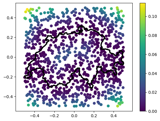
That was much faster, wasn’t it? We’ll cover hierarchical data structures in another tutorial. For now, let’s just learn that it’s a way to make our distance computation faster.
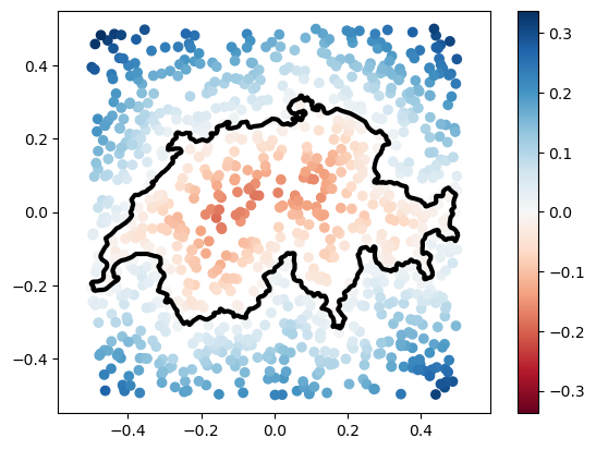
However, some times, distances on their own are not enough. A very common representation used today is Signed Distance Functions. These measure the same distance we measured above, but add a minus sign if the point is inside the polyline. It may be tempting to think that, by computing unsigned distances like above, we’re already 90% of the way there to signed distances. However, it turns out that reliably computing the sign of a given query point (this is known sometimes as an inside/outside query) is far from trivial. Fortunately, gpytoolbox can do it for us, and it will already use an AABB tree by default:
# Compute signed distances
from gpytoolbox import signed_distance
sdist, ind, t = signed_distance(points, vertices, F=edges)
# Plot signed distances and polyline
_ = plt.plot(vertices[:, 0], vertices[:, 1], '-k', linewidth=3)
_ = plt.scatter(points[:,0], points[:,1], c=sdist, cmap = 'RdBu', vmin = - np.abs(sdist).max(), vmax = np.abs(sdist).max()) # using a divergent colormap and centering it makes sense for signed distances, where "zero" is the surface
_ = plt.colorbar()
_ = plt.axis('equal')
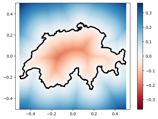
Often, you will want to compute these distances for all the points in a grid, which we can construct using numpy and gpytoolbox:
# Build a grid
x = np.linspace(-0.5, 0.5, 100)
y = np.linspace(-0.5, 0.5, 100)
X, Y = np.meshgrid(x, y)
points = np.array([X.flatten(), Y.flatten()]).T
# Compute signed distances
sdist, ind, t = signed_distance(points, vertices, F=edges)
# Plot grid with signed distances as color
_ = plt.pcolormesh(X, Y, sdist.reshape(X.shape), cmap = 'RdBu', vmin = - np.abs(sdist).max(), vmax = np.abs(sdist).max())
# Add polyline
_ = plt.plot(vertices[:, 0], vertices[:, 1], '-k', linewidth=3)
_ = plt.colorbar()
_ = plt.axis('equal')